- llm-inference
- deep-learning
Can a Language Model Reason in Fewer Tokens?

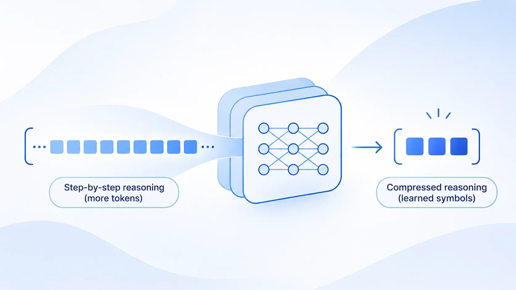
A language model solving a math problem often writes out the working before giving an answer (Wei et al., 2022). These reasoning tokens work like a scratchpad: each intermediate step becomes context for the next. Models typically learn this habit through supervised fine-tuning on worked solutions: each training example is a question, a step-by-step solution, and a final answer, and the model learns to predict the solution one token at a time. But how much of that working needs to be written in words?
What if we could replace a chunk of it with a single learned symbol—and still reach the right answer?
Token Assorted, by Su et al., explores exactly this question. We recreated its mathematical reasoning pipeline in our unofficial implementation, teaching a model to mix compressed symbols with ordinary text. The paper reports accuracy gains from this approach. In our recreation, models trained with latent codes produced shorter responses but lost some accuracy against text-only reasoning baselines, so we could not reproduce those gains.
This blog is for ML engineers, researchers, and readers familiar with language models who want to understand latent reasoning in practice. We’ll walk through how we recreated it, one training stage at a time: the choices that helped, the ones that fell short, and where the accuracy–length tradeoff ended up. Along the way, we’ll flag what we would check first if we started over. These checks may help in your own experiments too.
Why shorten the scratchpad?
Writing a solution step by step gives a language model a scratchpad. It also requires generating more tokens. Latent reasoning methods often explore whether learned representations can carry some of that intermediate work more compactly.
There are several ways to teach models to work through problems. Chain-of-thought (CoT) prompting puts worked examples in the prompt. Supervised fine-tuning on scratchpads trains the model on question → reasoning → answer examples. Reinforcement learning can reward successful attempts, for example by checking the final answer. Our implementation uses supervised fine-tuning, as proposed in the paper.
The next choice is how to represent that scratchpad. Coconut, for example, feeds continuous hidden states back into the model. Token Assorted uses a discrete alphabet of learned codes that can join the ordinary vocabulary. The model can then learn to predict codes and text using the same next-token training objective.
That leaves two jobs: learn useful codes, then teach a language model to reason with them.
Where we started: build an alphabet, then teach a model to use it
The training pipeline has two stages. In Stage 1, we train an autoencoder that compresses chunks of reasoning text into learned codes. In Stage 2, we fine-tune a language model on reasoning that mixes those codes with ordinary text.
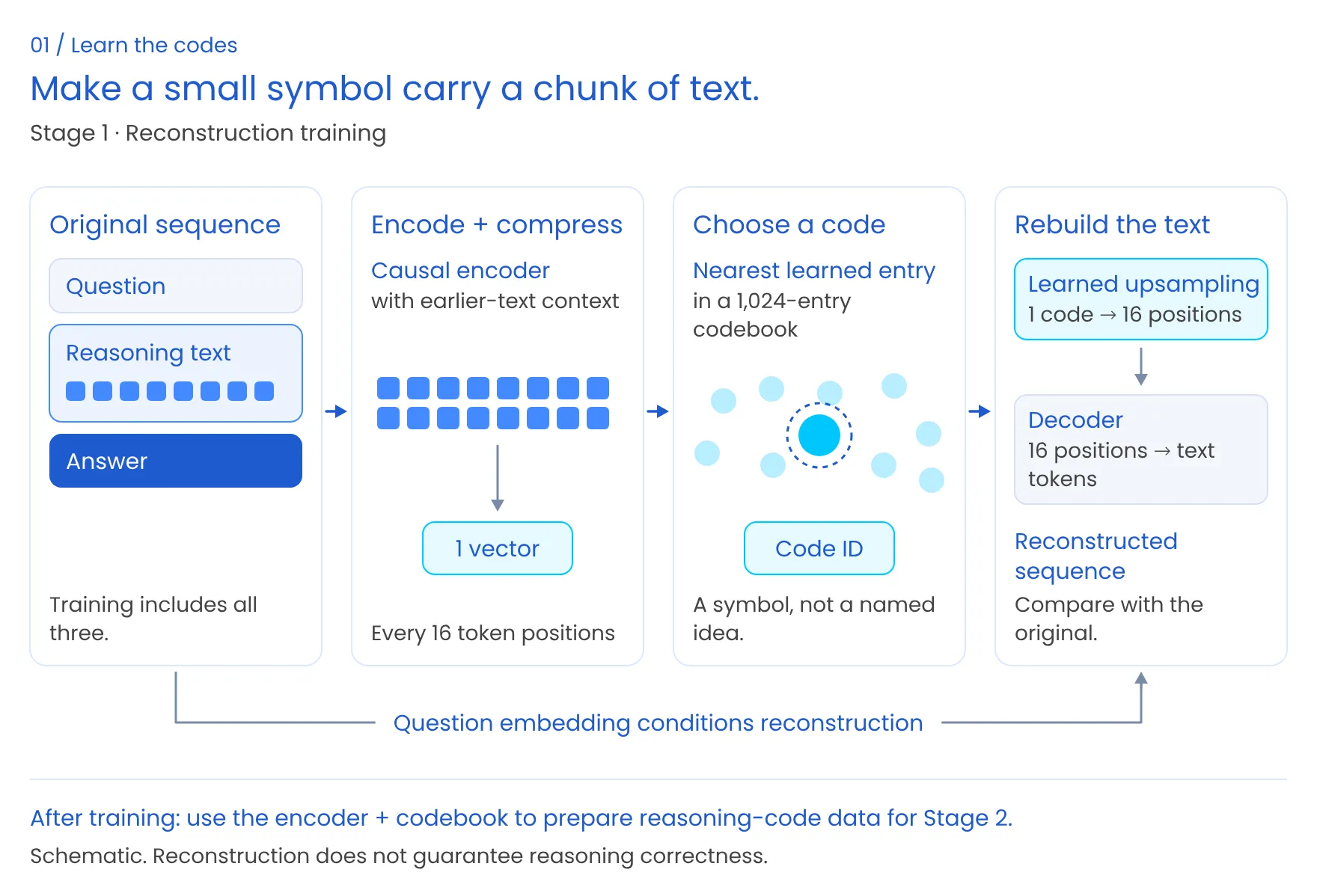
Stage 1: compress and reconstruct. A vector-quantized variational autoencoder (VQ-VAE) learns to encode text into compact representations (codes) and decode them back into text. Following the paper’s math setup (Section 4.2), every 16-token chunk becomes one of 1,024 learned codes. The encoder compresses each chunk into a vector, then selects the nearest vector in a learned lookup table called the codebook.
Training examples contain the question, reasoning, and answer. The decoder tries to recover the text from the codes and question context; later, the codes substitute for reasoning text. Each code identifies a learned vector—it has no guaranteed human-readable meaning such as “add these numbers.”
Stage 2: mix codes with text. As in the paper (Sections 3.2 and 4.2), we extend the LLM’s vocabulary with the codes and two markers that delimit a block of them. For each training example, we replace an initial portion of the reasoning with codes, keeping the question, remaining reasoning, and answer as text. The replacement length varies in whole chunks (16 tokens), including examples with no replacement.
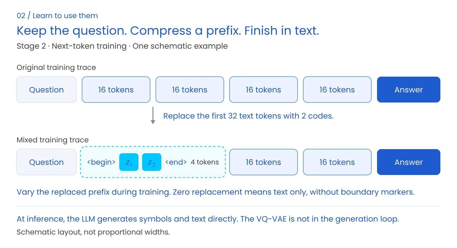
After training, the LLM generates both codes and text itself; the autoencoder’s (from Stage 1) job is already done. The 16:1 compression applies to replaced chunks: 16 natural-language tokens are replaced by a single learned latent token. We use the same compression ratio as the paper. Whole responses still contain text and boundary markers, so that ratio does not imply a 16× reduction in response length or serving time. See the paper’s method and experiments.
For the LLM trained with latent codes to work, the codes need to preserve the useful information; Stage 1 training enables that.
The first trap: a decoder can look good for the wrong reason
Our first decoder was autoregressive: it predicted text one token at a time. During training, we used teacher forcing, supplying the correct preceding tokens at each step.
That made reconstruction look encouraging. It also gave the decoder a shortcut: it could use the preceding words to predict plausible continuations without relying enough on the codebook. A good reconstruction score alone could hide weak use of the codes.
We tried dropping some decoder inputs to reduce that dependence (dropout). Higher dropout improved codebook usage to some extent, but it made the decoder’s output loop and repeat. The more useful change was a parallel decoder, which reconstructed the text from the codes and question context without seeing the correct text prefix. Reconstruction became harder, but the test became more informative.
We also checked encode–decode round trips: compress the reasoning, decode it, and inspect whether the original numbers survived. Dropout hurt here too: the autoregressive decoder trained with dropout preserved fewer of the original numbers. A mathematical explanation can sound fluent even after its quantities have changed. That is an expensive failure to discover only after training the LLM.
Next came the codebook. Our reliable Stage-1 recipe initialized it from encoder outputs, used exponential moving average (EMA) updates to blend new observations into existing entries, and replaced unused entries more conservatively with a grace period after each reset. EMA worked slightly better in our experiments than gradient-based updates for the codebook.
With the codebook sorted, we turned back to the decoder and to one step in particular: how a single code expands back into sixteen positions.
The biggest gain came from expanding a code
Our Stage-1 autoencoder used Transformer blocks from Searchformer. The first parallel decoder prepared its input by copying each selected codebook vector across 16 positions. We replaced that repetition with a learned upsampler, which learns a separate transformation for each position within the chunk.
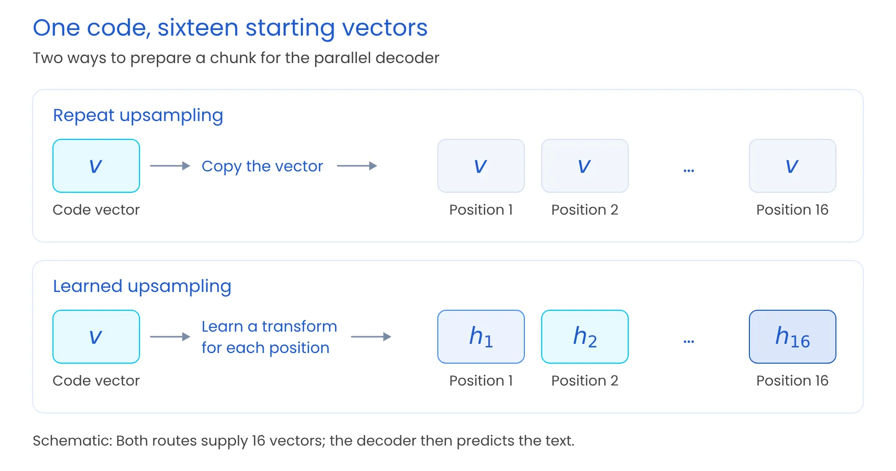
That change produced the clearest retained improvement in Stage 1:
| Measurement | Repeat upsampling | Learned upsampling |
|---|---|---|
| Reconstruction token accuracy | 30.59 ± 0.17% | 47.35 ± 0.10% |
| Numbers retained in a round trip (encode → decode) | 15.5 ± 0.4% | 46.7 ± 1.7% |
Number retention rose from 15.5% to 46.7%. The decoder was recovering substantially more of the original quantities, although even the improved result left plenty of room for information loss.
The values are in mean ± standard deviation format, measured across three seeds. Reconstruction accuracy covers held-out full sequences. Number retention measures the fraction of distinct original numbers recovered when decoding the CoT part of the sequence from its codes, using 100 held-out examples. Retaining a number does not establish that the model used it correctly in arithmetic.
We also tried plain Transformer blocks in place of the Searchformer blocks. That variant came close, but learned upsampling with Searchformer blocks remained our best of these tested configurations. The full comparison, including this variant, is in the Stage 1 results table in the repo README.
The practical lesson was to inspect how the decoder uses and expands the compressed representation. But the next test was more demanding: could a language model use these improved symbols to solve problems?
Next: teaching a language model to read the alphabet
A new code needs a numerical representation inside the LLM—an embedding. We explored how to initialize these embeddings and whether to tie the embedding layer and the output head, so the same weights are used for reading and predicting tokens.
Starting every code from one shared vector, the average of the existing token embeddings, worked poorly: the codes stayed nearly identical even after training, far more alike than ordinary tokens are, so the model had little to tell them apart by. Giving each code its own starting vector improved in-domain accuracy a few points. Untying the layers added nothing.
Our best recipe therefore starts each code’s embedding from the average embedding of the text chunks assigned to it and keeps the layers tied, then fine-tunes the whole model. This gives each new symbol a distinct starting point based on the text it replaces.
Last came evaluation. We made training deterministic and moved evaluation from bf16 to fp32, a higher-precision numerical format, after observing results change with batching in bf16. These numerical accuracy issues can complicate comparisons between training choices.
With the pipeline in place, we could test the outcome that mattered: answer accuracy alongside response length.
Shorter responses came with an accuracy cost
We evaluated on GSM8K, a collection of grade-school math word problems, and MATH, a competition-math benchmark. Both are in-domain datasets: we used them to construct our training data, and the results below are on unseen problems. Results on other, out-of-domain datasets show similar patterns. “Latent” means mixed code-and-text reasoning; CoT is the matched text-only reasoning baseline. The table shows representative results; see the Token Assorted release README for more details.
| Model / benchmark | CoT accuracy | Latent accuracy | Generated tokens, CoT → Latent |
|---|---|---|---|
| Llama-3.2-1B / GSM8K | 46.3% | 40.8 ± 0.7% | 120.0 → 101.8 ± 3.4 |
| Llama-3.2-1B / MATH | 12.1% | 10.5 ± 0.2% | 164.0 → 135.8 ± 10.9 |
| Llama-3.2-3B / GSM8K | 65.0% | 61.1 ± 0.3% | 123.2 → 104.0 ± 1.8 |
| Llama-3.2-3B / MATH | 19.0% | 17.5 ± 0.6% | 210.1 → 139.5 ± 7.5 |
The Llama-3.2-3B result on MATH makes the tradeoff concrete: average output length fell from 210.1 to 139.5 tokens, while answer accuracy fell from 19.0% to 17.5%. The other rows tell the same story. We also ran the experiments on the instruction-finetuned (Instruct) variants of these models, which are further trained to follow instructions. These also produced shorter responses with lower accuracy than their CoT baselines on GSM8K and MATH.
A few details matter when reading those numbers. The latent values summarize three seeds that vary which reasoning prefixes are replaced. CoT runs are identical across those seeds because their training data does not change. Training uses one epoch; evaluation uses greedy decoding—choosing the highest-scoring next token—and the official benchmark scorers.
Output token counts include latent tokens and the end-of-sequence marker, with generation capped at 512 tokens. These results measure response length under that budget, not model serving latency.
Better reconstruction had not closed the downstream accuracy gap. These experiments do not isolate why that gap remained; they show why recovering text and solving the original problem need separate tests.
Conclusion: what reproduced and what didn’t
We reproduced the training pipeline and got the shorter responses (11–36% fewer generated tokens than CoT, against about 20% in the paper), but not the accuracy gains: where the paper reports +4.1 to +6.0 points on GSM8K and +4.2 on MATH, our Latent models landed 3.9–5.5 and 1.5–2.5 points below CoT. What worked for us was a parallel decoder, a learned upsampler, an EMA codebook, and initializing each code’s embedding from the text it replaces. What did not was a teacher-forced autoregressive decoder, a shared starting embedding for all codes, untying the embedding layer from the output head, and plain Transformer blocks; better reconstruction alone did not close the accuracy gap. Our setup differs from the paper’s in some places; these differences and the full result tables are in the repo README.
What to take into your next experiment
Our implementation turned the idea of a shorter reasoning alphabet into a working pipeline. The experiments also changed what we would check first:
- Check what survives compression. Inspect decoded reasoning and its quantities alongside aggregate reconstruction scores.
- Check what the decoder can infer without the codes. Access to the correct preceding text can make a weak compressed representation look more useful than it is.
- Measure answer accuracy and response length together. Improvements in the autoencoder need to earn their place in the final reasoning model.
We’re releasing both training stages, code extraction and reconstruction tools, CoT and answer-only baselines, and benchmark evaluation. The README contains the setup instructions and complete result tables for exploring these choices yourself. If you find a fix, a better recipe, or a new experiment worth adding, we welcome contributions: open a pull request on the repo.
 Explore Token Assorted on GitHub