
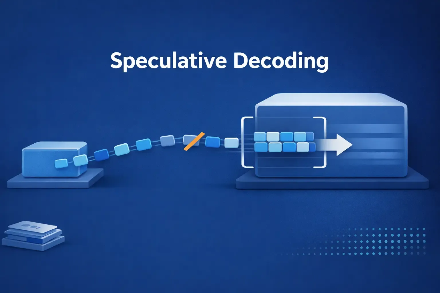
Speculative Decoding
Introduction
Large Language Models (LLMs) power many of today’s AI systems, but their inference is slow and costly because text is generated one token at a time, with each step bottlenecked by GPU memory bandwidth. While techniques like quantization, pruning, and distillation aim to speed things up, they usually require altering the model itself. Speculative decoding takes a different approach: it pairs a smaller, faster model that “guesses ahead” with a larger model that verifies those guesses in bulk, offering a practical way to accelerate inference without sacrificing accuracy.
How Do LLMs Generate Text?
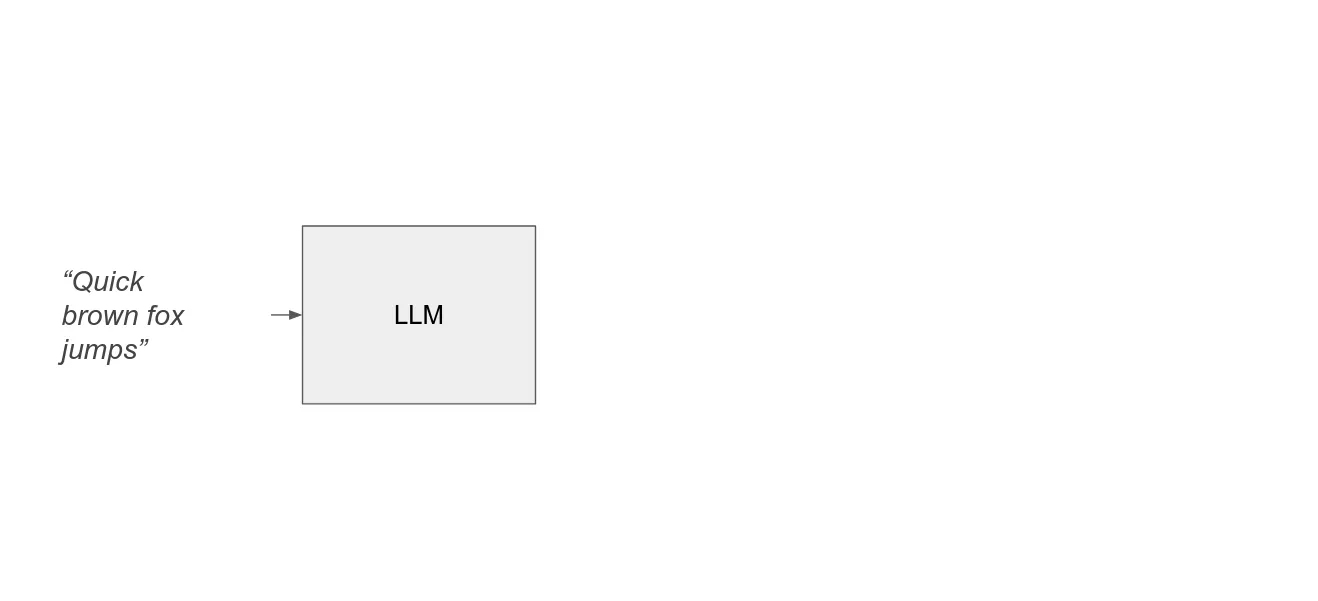
Whether you are prompting an LLM to classify text or generate a poem or answer a query about your dilemmas, the LLM generates new text as a response to your query. It generates the text one token at a time. At each step, it will consider the text that you had initially provided and the text that it has generated so far as its input to generate the token for the given step.
 |
|---|
| Fig 1: Visualization of Auto-Regressive Generation |
At each step, the model not only outputs the next token but also updates its internal hidden states. This detail becomes crucial when we later talk about how speculative decoding verifies tokens efficiently.
Why is LLM Inference Slow and Expensive?
LLMs generate outputs one token at a time. This is called Auto-Regressive decoding. Each new token generated by the model requires a full pass of the entire model. GPUs are extremely fast at computation, but that speed doesn’t translate to fast generation because the real bottleneck is memory access. Each step involves moving large tensors and reading model weights from GPU memory, and that memory bandwidth becomes the limiting factor.
To make inference faster, most optimization methods focus on reducing how much data needs to be moved. This is usually done either by shrinking the model itself or designing smaller alternatives that require less memory traffic.
Existing Optimizations
Many existing optimizations exist to improve LLM’s inference. Most of these revolve around reducing the model’s memory.
Quantization is one of the most popular ways to reduce the model’s memory footprint. Instead of storing model weights as 32-bit floating-point numbers, we can compress them to lower-precision formats like 16-bit or even 8-bit. That instantly cuts the memory footprint in half or more, which reduces memory bandwidth requirements during decoding. A more aggressive push in this direction is BitNet by Microsoft, which represents each weight using roughly 1.5 bits on average through ternary or binary-like encodings. The core goal of quantization is to shrink the amount of data that needs to be stored and moved, without destroying model quality.
Another major memory and compute bottleneck in LLMs is the attention mechanism. LLM is made up of many attention heads, which are essentially large 2-dimensional matrices. Each layer contains multiple attention heads that compute interactions between every pair of tokens in the sequence in the form of 2-dimensional matrices. This results in quadratic memory and computational cost. The computation required for these attention matrices is of quadratic time and memory complexity. Techniques like Flash Attention optimize how the attention mechanism works under the hood. Although the Flash Attention does not require changing the model’s architecture, it still requires a rewrite of the attention kernels of a given model.
Shallow Decoding is another such approach, which involves reducing the size of the Decoder (in case your LLM follows the Encoder-Decoder architecture).
Most of these optimization techniques come with two major drawbacks. First, they require changing the model’s architecture or implementation, which means you can’t just apply them to a model out of the box. Second, they often trade speed for quality—smaller or heavily modified models rarely match the performance of the originals. This leads to an obvious question: can we speed up inference without touching the model itself?
Enter: Speculative Decoding
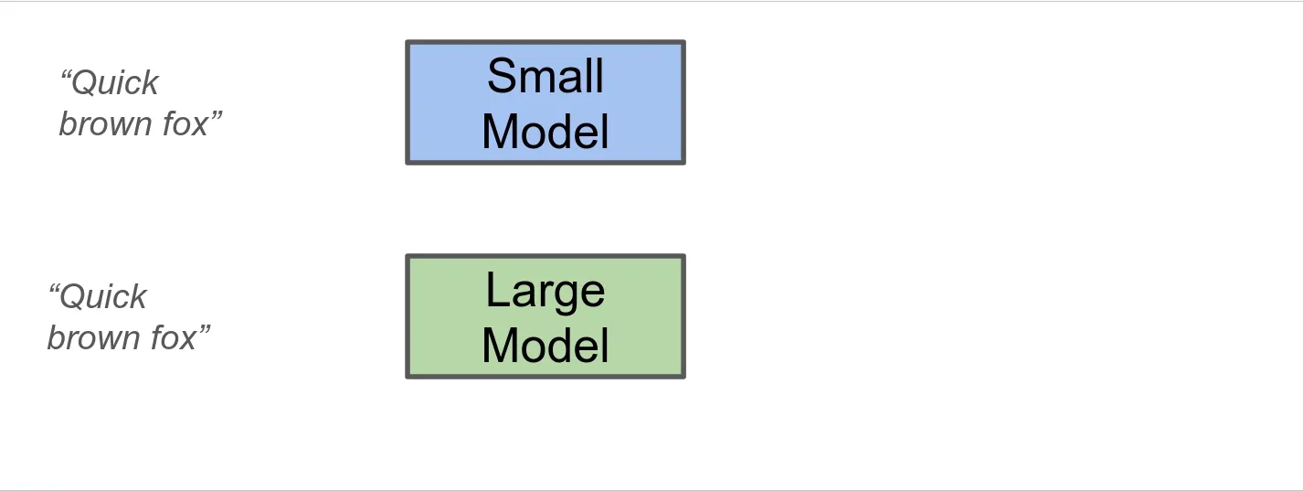
So far, we’ve seen that larger models take longer to generate each token, while smaller models can produce tokens much faster. That difference is exactly what Speculative Decoding takes advantage of.
 |
|---|
| Fig 2: Difference in Inference Speeds of Small and Large Models |
Instead of asking the large model to generate every token one by one, we let a smaller “draft” model predict the next few tokens—say, K of them—all at once. Then, we pass those K tokens to the large model in a single step to check whether it would have made the same predictions. If the tokens match, we accept them and move on. If not, we fall back to the large model and continue from there
This means we replace K forward passes of the large model with K cheap passes of the small model plus one verification step from the large model. Even with occasional corrections, this can be much faster than having the large model generate every token itself.
 |
|---|
| Fig 3: Generating Outputs Speculatively |
Speculative Decoding Concepts
Verification of Speculated Tokens
Any Large Language Model fundamentally predicts the next possible token given a sequence of input tokens. When we provide the model with an input, say “Quick brown fox,” it answers the following questions,
- What is the next probable token given input “Quick”?
- What is the next probable token given the input “Quick brown”?
- What is the next probable token given input “Quick brown fox”?
As the end user, we are only concerned with the answer to 3.) What is the next probable token given input “Quick brown fox”? However, the model will internally calculate answers 1 and 2 as well. These are the Hidden Probability States calculated by the model. These Hidden Probability States hold the key to verification
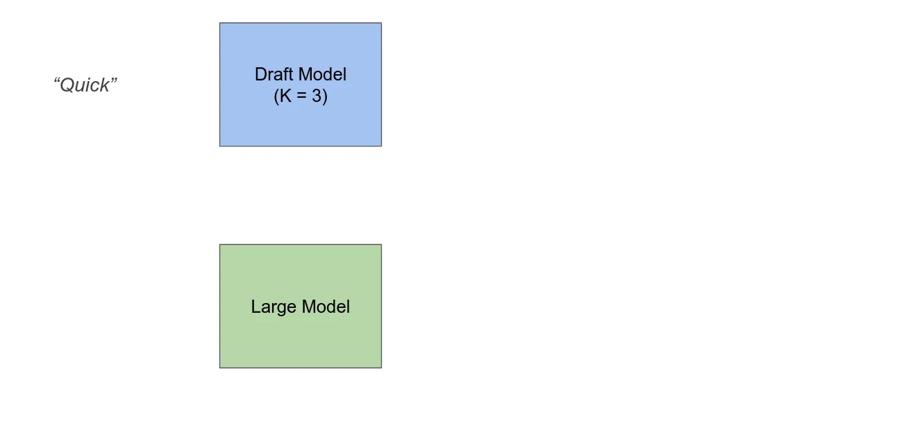
Speculation Step
Let’s say we start with the following input “Quick”, we pass it to our Draft Model with K = 3. This will result in the following outputs from the Draft Model,
“Quick” → Draft Model → “brown fox jumps”, K=3
Verification Step
We pass the Input + Draft Tokens from the Draft Model as input to the Large Model
“Quick brown fox jumps” → Large Model →
The Large Model will then produce Hidden Probability States as follows,
- PLarge(T1 | “Quick”)
- PLarge(T2 | “Quick brown”)
- PLarge(T3 | “Quick brown fox”)
- PLarge(T4 | “Quick brown fox jumps”)
The Output given each input sequence can be computed by sampling from the predicted Hidden Probability State.
- Max(PLarge(T1 | “Quick”)) → brown
- Max(PLarge(T2 | “Quick brown”)) → fox
- Max(PLarge(T3 | “Quick brown fox”)) → jumps
- Max(PLarge(T4 | “Quick brown fox jumps”)) → over
 |
|---|
| Fig 4: A deeper look into how LLM generates its output along with hidden states. Note, for illustration sake, we’ve shown hidden states and output generated separately, but internally, it all happens in one single run. |
We can use this to verify the outputs that the Draft Model generated at each of the K Steps
| Step | Draft Model Output | Large Model Output | Is Accepted? |
|---|---|---|---|
| T1 | brown | brown | ✅ |
| T2 | fox | fox | ✅ |
| T3 | jumps | jumps | ✅ |
| T4 | N/A | over |
Given that the Large Model would have generated exactly the same outputs as the Draft Model, given the same inputs, we have successfully verified the outputs of the Draft Model in a single pass of the Large Model. This is much faster than generating all 4 tokens by the Large Model.
Handling Mis-predictions by Draft Model
In the above example, we saw that the Draft Model correctly produced all the K tokens as they would’ve been produced by the Large Model. What happens if it makes a mistake?
Again, we consider the same example
“Quick” → Draft Model → “brown dog jumps”, K = 3
The Large Model calculates the following probabilities,
- PLarge(T1 | “Quick”)
- PLarge(T2 | “Quick brown”)
- PLarge(T3 | “Quick brown dog”)
- PLarge(T4 | “Quick brown dog jumps”)
We can now compute the Outputs at each step,
- Max(PLarge(T1 | “Quick”)) → brown
- Max(PLarge(T2 | “Quick brown”)) → fox
- Max(PLarge(T3 | “Quick brown dog”)) → skips
- Max(PLarge(T4 | “Quick brown dog jumps”)) → over
We can now verify our Outputs
| Step | Draft Model Output | Large Model Output | Is Accepted? |
|---|---|---|---|
| T1 | brown | brown | ✅ |
| T2 | dog | fox | ❌ |
| T3 | |||
| T4 |
Here we see that the second token T2 predicted by the Draft Model was not what the Large Model would’ve predicted; we reject the remainder of the draft sequence and keep only the valid token plus the token the Large Model would’ve generated. In this case, we’ve only generated 2 tokens, i.e, brown fox. |
 |
|---|
| Fig 5: Visualising a single speculation step with correct as well as incorrect predictions. |
How to Select Draft Models?
Shared Vocabulary Requirement
The Draft Model must have the same vocabulary as the Large Model. Since the speculated tokens need to be verified by the Large Model, they cannot be from a different vocabulary. To ensure this, we usually pick Draft Models from the same Model family, e.g, if you’re using GPT-2-XL as your Large Model, you’d use the base GPT-2 as your Draft Model.
Size Requirement
The Draft Model you pick should be significantly smaller than the Large Model; otherwise, you might end up spending the same time speculating tokens from the Draft Model as you would’ve if you directly generated them from the Large Model. Ultimately, we want to speed up inference of the Large Model, and if the Draft Model takes almost the same time as the Large Model, we will not be achieving any speedups.
Draft Model Approximates The Large Model Well
This is another important requirement. If most tokens generated by your Draft Model are incorrect, you will be spending the same, or even more, amount of time generating the output. To ensure this, people usually try to use distilled or quantized versions of the Large Models as Draft Models. The figure below represents what happens if your Draft Model doesn’t approximate your Large Model well.
Challenges With Speculative Decoding
Hosting Two Models Together
One of the main challenges is that we need to have both the draft and large models hosted simultaneously to perform Speculative Decoding. This means increased costs in terms of infrastructure requirements for running both models.
Ensuring Efficient Implementation
The underlying implementation of the Speculative Decoding algorithm should ensure that the implementation itself is not a bottleneck. Naive implementations using token-by-token verification loops should be avoided. Also variable-length sequence makes implementation too complex.
Tight Verification Strategy
In the above examples, both the Draft Model and the Large Model samples verify tokens based on their maximum probability values; however, in practice, there are different sampling strategies that are used. Any verification strategy should be aligned with the underlying sampling strategy in the Draft and Large model.
Medusa Architecture: Beyond Speculative Decoding
Speculative Decoding works by speculating K tokens by a Draft Model and then verifying by the Large Model. This presents a set of challenges as discussed above, which makes Speculative Decoding itself a complicated system to implement.
If we take a look at how LLM works, broadly, they have two parts,
- The Attention Mechanism - This captures the interaction between different tokens.
- The Language Model (LM Head) - This determines which should be the next token based on the output of the Attention Mechanism.
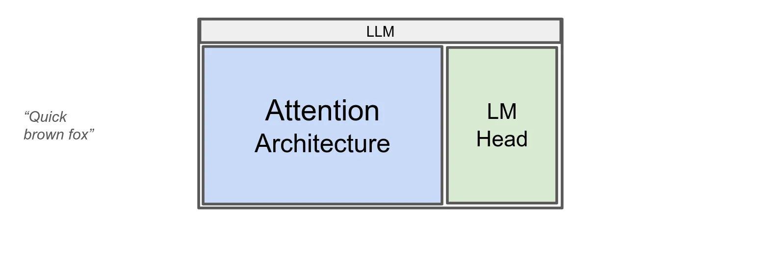 |
|---|
| Fig 6: Simple LLM Architecture Breakdown |
The reason why we generate only one token in the output is that we have only one Language Model head.
Medusa is an alternative architecture which suggests that rather than having one Language Model head, we can have K LM heads that can predict the next K tokens. This is the Generation Step. Just because we can generate the next K tokens in parallel does not mean the generation will be precise. This is because when we predict tokens in the future, the error increases as we predict further down the timeseries. Therefore, we need an extra step called the Verification Step. This step is exactly the same as the verification step in the Speculative Decoding algorithm. We take the outputs of all the LM Heads, pass them through the LLM, and verify them using our Hidden Probability States.
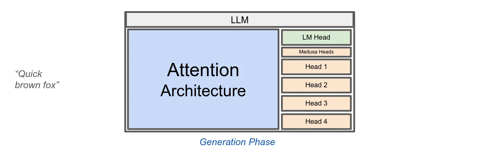 |
|---|
| Fig 7: Medusa Architecture. The Outputs of Medusa Heads are ignored during the Verification Phase. |
Conclusion
We’ve discussed how the traditional way of doing inference in LLMs slows down their speed at generating output. We unpack how the size of the LLMs is a major factor, slowing down the inference. We have also done a brief overview of methodologies around memory and architectural optimizations that help in speeding up LLM inference.
We build the intuition of how Speculative Decoding can improve inference speeds without changing the architecture of the model. We’ve also discussed how Speculative Decoding is implemented and what the common issues are that one might face while implementing it. At the end, we talk about the Medusa architecture, which builds upon the concepts of Speculative Decoding and improves upon it.