Classify Between Breeds of Dogs

Classification of breeds of dogs is a very popular problem in machine learning where our system would predict the breed of a dog given its picture. This problem falls under fine grain classification problem where the objects generally differ only in very tiny features which are difficult to differentiate. In this blog i will share my approach and results for this problem, so lets get started.

For this problem we will consider the data collected by Stanford Dogs dataset . This dataset contains total of 20,580 images of dogs varying across 120 dog breeds. There are roughly 200 images per breed. The dataset is well varied from breeds across the globe. This dataset has been built using images from Image net for the task of fine grained image categorisation. We will be downloading our data from the kaggle problem from here. The data has been taken from Stanford dataset and has the following files. It contains a Train folder with 10222 images of dogs which can be used for training. The Test folder contains about 10357 images for testing. The labels.csv file contains the 10222 values with class labels for each training data image.

It is always a good idea to do some data analysis for our data.

lets start by seeing our distribution of data across different classes.

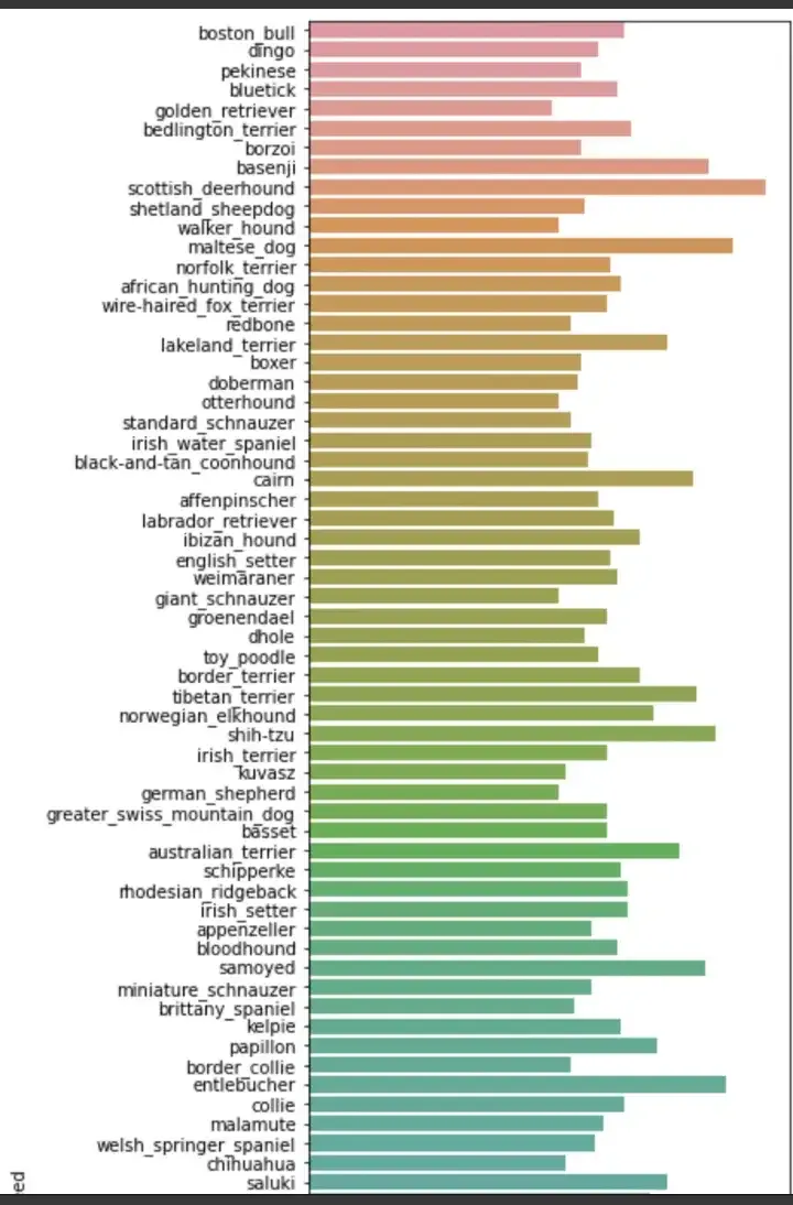
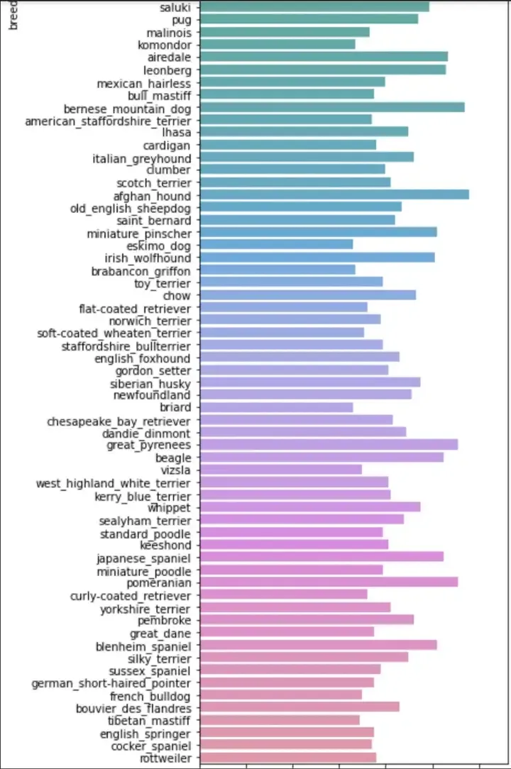
As seen from the above plots we can see that our data is fairly evenly distributed across each class and there is not much of a problem of unbalanced data. This looks Good.

Since this is CV problem we need to find a fixed image size for our input to the model. To get an idea about this it is beneficial to have a look at distribution of heights and widths of images in our training data.

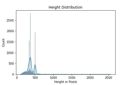
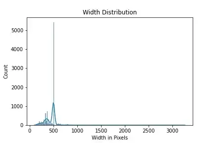
Above plots gives us an idea of height and width of images in our dataset. We can say that 90% of our data has width less than 500 pixels, based on our compute power we can set our height less than 500. Similarly we can say that most of our input width is around 500, based on these info we can choose different input sizes eg (256,256),(300,300),(400,400) with upper limit of 500 for both width and height.

Lets have a look at the distribution of mean pixel values in our training data.

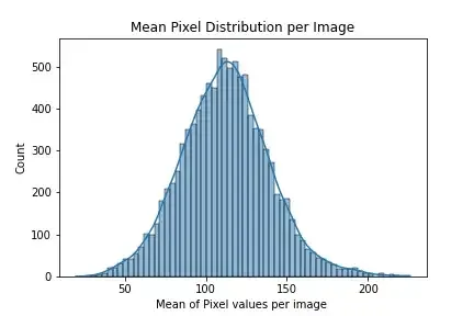
From the plot above we can see that our mean pixel values follows a normal distribution with mean at 110.

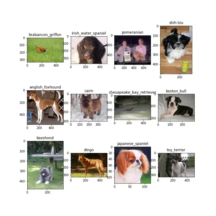
Next, it is always good to look at the actual images when dealing with CV problem. Let us look at images of some classes of dog selected at random.

Above we have random selected images for dog breed golden retriever, as we can see that most images look identical apart from some where we have puppies also. Next we can have a look at the mean image for this class.

Seeing the mean image we can see that our dog is well centered across all images and is predominantly of blue colour in the images.

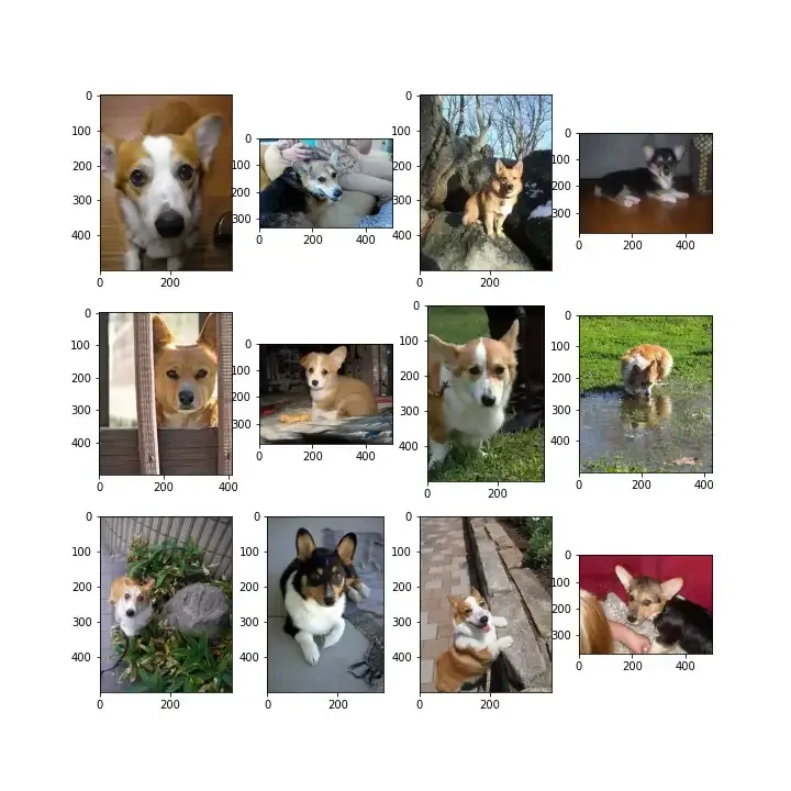
Lets see some randomly selected images from our dataset

we can see that across our dataset our images are sometimes challenging as images are very varied in terms of dogs being in different regions of image.

To solve this problem i used transfer learning as my main approach , in which i tried different pretrained models as my backbone. In general i used a pretrained model on imagenet data and used it as my backbone which would give me vector representation for my input image. This representation was then used in our model head which was generally single layer MLP connected to a softmax. This model head was then trained on the training data keeping the backbone fixed (no training) and results were inferred once the model was trained.

I basically used Inception as my main backbone. The first model used was simple inception V1 as backbone followed by a 2 layer MLP head with 1024 and 120 units each. Below is the summary of the model

I started training this model with learning rate of 0.003 for Adam on input size of 256,256. I got a validation logloss of 1.14 with validation accuracy of 0.70. Here are my training plots.

As we can see that our validation loss is not improving much for each epoch , may be we need to change the architecture of our head to improve it further.

Next i tried same model with a different learning rate of 0.0001 with same image input size. I got an improved validation score of 0.87 and validation accuracy of 0.72. Got some improvement.

Next i tried same model with a learning rate of 0.001 with input size of (400,400). In this case i got val score of 0.72 and val accuracy of 0.77.Below is the training plot.

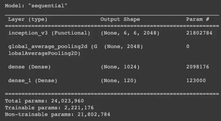
Next model which i tried was with the same inception v1 backbone but with changed head. This time i increased the learning capability of my head so i used a 3 layer MLP with 1024, 512 and 256 units followed by a 120 unit softmax. Here is the summary.

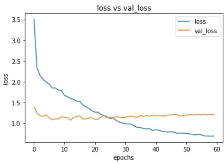
I trained this model with lr of 0.001 with input image sizes of 400,400. The val logloss that i got was 0.70 with val accuracy of 80%. Here are my training plots.

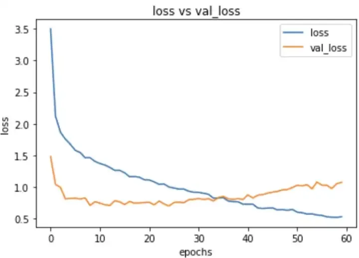
In this case we can see that our val loss is not reducing with epochs and has plateaued after initial epochs.

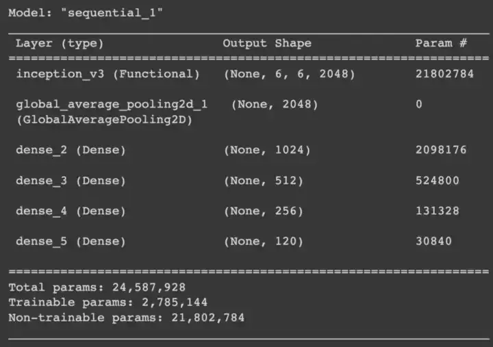
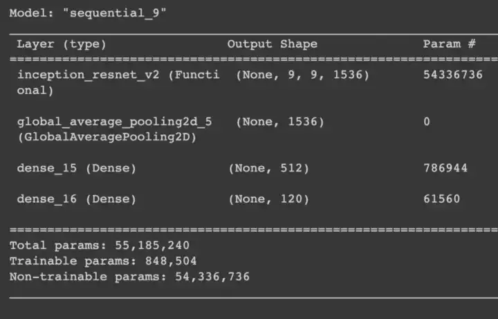
In all our previous models we can see that our models has fairly large number of trainable parameters as compared to the number of data points we are having. To make this better i tried a much smaller head this time with dropouts in between the mlp. Also in this case i will be using InceptionResnet v2 as my backbone. I used a 1 layer MLP with 512 units followed by a softmax along with a dropout of 0.3 between them. Here is the model summary

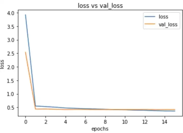
I trained this model with the input size of 350,350 , started by lr of 0.001 the reducing it to 0.0005 after half epochs were reached. i got a validation loss of 0.5 and validation accuracy of 86%. Here are the training plots for the same

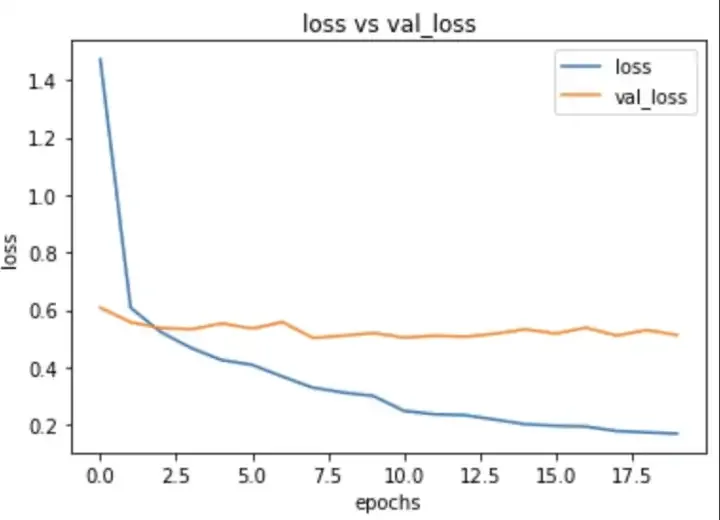
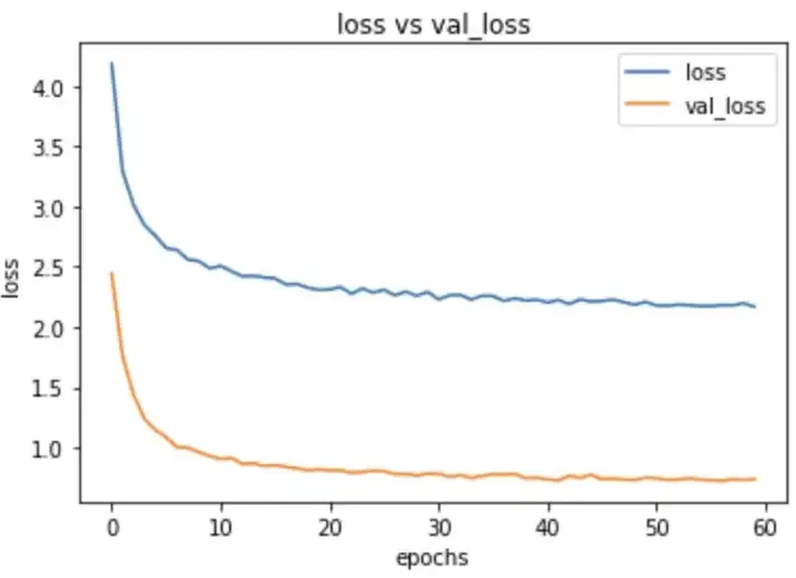
Next i tried the same model , but changed my learning rate, i started with lr of 0.0001 and also with increased image size of 400,400. This model outperformed all my previous models and gave a validation loss of 0.41 and val accuracy of 86%. Here are my training plots for the same.

As you can see that this plot really looks good as there is very less sign of overfitting in our model.

There were several other approaches that i tried but this was my best performing model. Also with more thinking it is possible to achieve very low loss for this problem, but that remains a task for future for me.

Just to test our final model i randomly selected 20 datapoints from test data and predicted their breed using my model , here are the results that i got

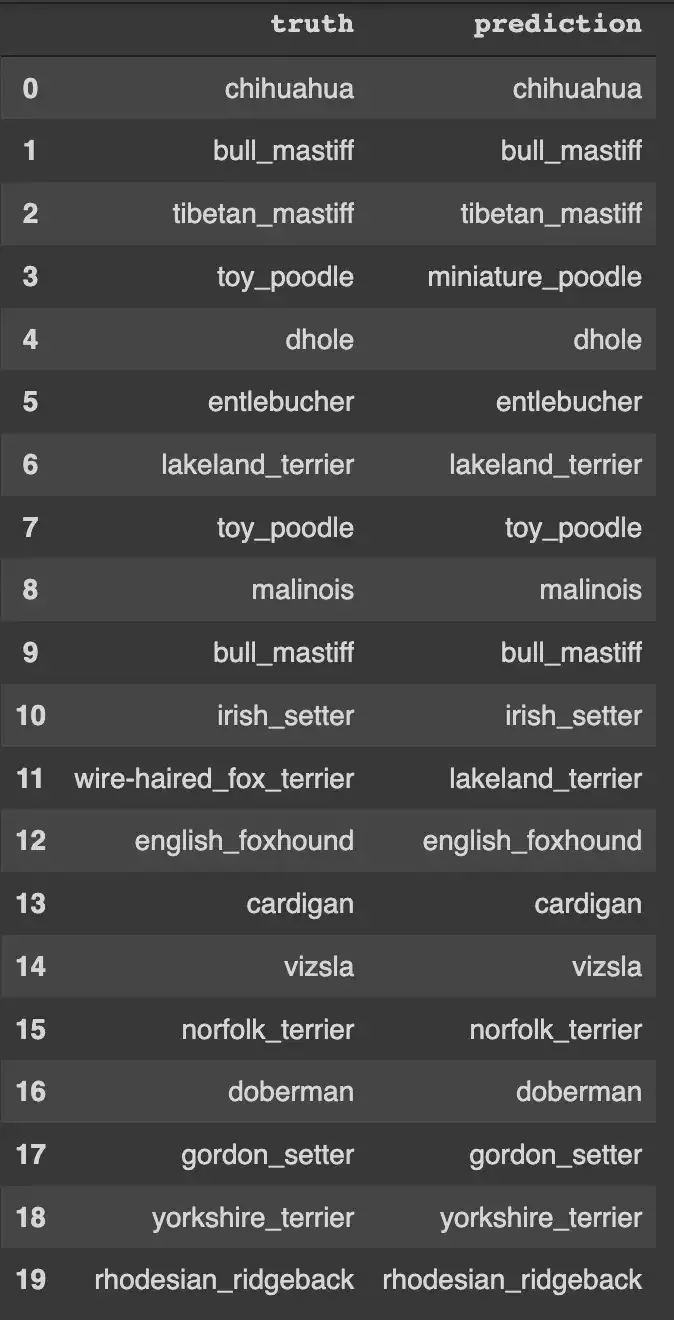
I ran the test multiple times and could see that model was able to give about 87% accuracy. Above picture shows the result of one such iteration.

Now since this was a kaggle problem i also tested this model on the kaggle test data provided by them. This model performed fairly well and gave a log loss of 0.44. This loss can further definitely be reduced using different techniques.

In this section i am going to discuss some of the post training EDA done on the data . This method can be quite good in making our training data better and help us understand our model performance much better, so that we can take necessary actions required. We can generally improve performance of our model without changing the model itself, for this we just need to understand our data better and understand that for which datapoints our model is performing badly. Once such data points are classified , we can take actions to improve our data.

On similar lines , in order to understand our data better we will divide our data into 3 categories good, medium and bad. Once we categorize our data we can get an idea of the classes for which our data is not performing well. We can also use confusion matrix here to do the same, but the problem is that we have 120 classes with us and it will become difficult to visualize such big matrix.

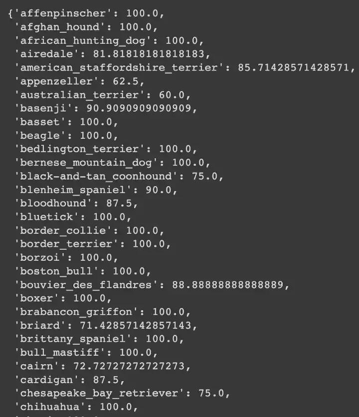
To divide our data, we will use accuracy as our metric, so idea is to predict dog breeds for each class in our test data. Then we would calculate accuracy for each class separately to get an idea about the class performance. Below we can see for some classes the accuracy i got.

A better way to get an idea about accuracy per class is to have a look in terms of distribution of accuracy, below plot shows the same.

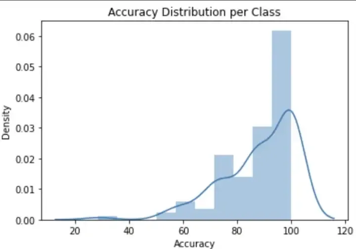
From the distribution we can see that most of our classes are getting correctly classified with accuracy of 100% , but still there is a fatter tail from 60 to 100, indicating that these are the classes for which our model is performing not that well. To distribute our training data we can define the ranges for accuracy, eg in my case i decided to put each data point belonging to a class into good category if the accuracy for that class lies between 85 to 100.

Similarly medium performing class were defined between 65 to 85 and poor performing classes were defined less than 65. We got 87 classes that are giving good accuracy , but there are 8 classes that are not giving good accuracy. so lets focus on these 8 classes.

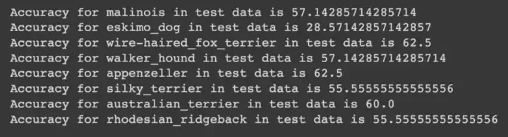
The above image shows us the 8 classes performing poorly in our dataset. Out of these 8 classes eskimo_dog has got the lowest accuracy of 28%, lets disect into this class in our data.

I tried to predict eskimo_dog class images from my test data and these are the results i got

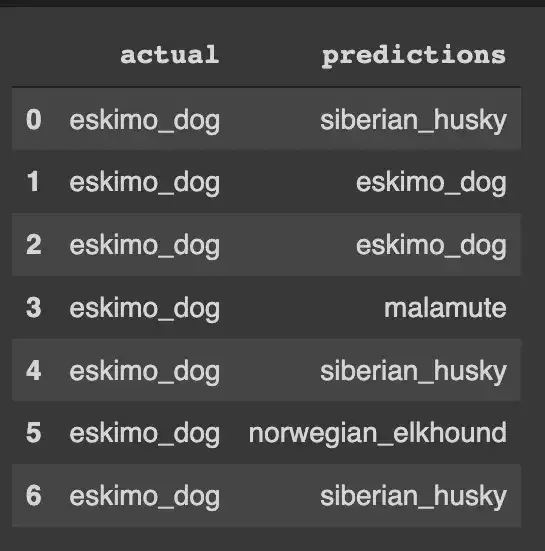
as you can see that the model is mixing eskimo dog with many different breeds. One thing we have to see is that though our model is predicting wrongly for the eskimo dog but still there is some common ground between all these dogs, as they all are believed to habitat in colder regions . so there is something that our model learnt . Now why our model is misclassifying ? well there could be many reasons for this maybe our data quality is not good for these classes, or it could be the case where it is actually quite difficult to differentiate between them.

Lets have a look at some of the sample images of eskimo dog and siberian husky (since it is mostly getting confused with) in our train data.

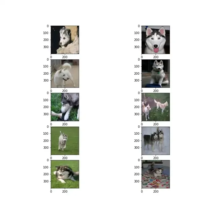
The left images are of eskimo dog and right images are of siberian husky. Now one thing we have to notice is that even to a human it would be difficult to differentiate between them in the given data. Images seem to be quite similar, so to be fair it could be a case where our data is good but the problem in itself is a bit challenging. In this case it will be wiser to look at our model for improvements, so that it can catch those fine grain differences also.

At last i deployed my best performing model locally on my machine using flask, below is the small video in which i randomly give it a dog image downloaded from internet and we can see that the model is predicting correct results.

It is to be noted that the model is taking way too long for predicting the output , however that i think comes down to the fact that i am using my machine to produce inference and i think it will improve on a better and faster machine.

To be fair we can still improve this model to classify well with similar looking breeds, for that we can shift our attention to using vision transformers . In future i would like to work with vision transformers for such fine grain classification problems because they seem to work really well in finding those small differences. For the code reference visit my github here. Feel free to connect on my linkedin.