Capsule Networks: Everything You See Is Not True
Expensive alternative to Convolutional Neural Networks (CNNs)
Today when we talk about data, we’re no longer confined to the traditional columnar or CSV-type data sources. There has been a rise in data of all formats and types ranging from sound to image data, from cross-sectional to time-series format due to better availability of data structures and methods to retrieve and store different kinds of data.
This article is rather focused on one such type of data, Visual data to be precise, and its context with Machine Learning. The foremost approach earlier to deal with Image data was to flatten the data into a vector and pass them into a Neural Network or some other Machine Learning algorithms for different purposes. With the development of Deep Learning, things took a drastic turn, and the world was introduced to Convolution Neural Networks (CNNs) by Yann LeCun in the late 80s. CNNs have proven to be the current state-of-the-art (SOTA) methodology for working with Visual data of all kinds ranging from images to continuous data like Video clips.
In the case of CNNs we just load the data and train the network to identify features in the 2D space which get tangled when flattened. With successive layers building up the network, the field of view of later layers keeps on increasing making it possible to learn more complex features. Yann LeCun demonstrated this concept by training a five-layer model on the MNIST dataset and classifying the digits with a 98.49% accuracy.
Despite being the game-changer in the field of Deep Learning, CNNs have inherent disadvantages that most people are unaware of. We’ll explore them now and that will help us build a base for the main topic of this blog: CapsuleNets.
Disadvantage #1
Due to their nature of capturing feature information for higher-level tasks such as classification, segmentation, object location, etc. they have been agnostic to the position and/or the orientation of those features. When we hope for them to learn the distribution of a dataset, they rather focus on the training images supplied to them.
Disadvantage #2
Given the above limitation, CNNs are however agnostic to the relative positions of these features also. While moving upward in the layers, they only capture what features are present in the image to perform their task. This limitation arises due to the structural issues in any CNN architecture.
In CNNs, we often use pooling layers to reduce the image size or to cut down the computational burden, but what we don’t think is that by averaging or taking the pixel with the highest values we’re losing a lot of positional information about that feature. Also, by choosing the one with the highest value, we’re basically sub-sampling the features from the image.
Focus on the image below to better understand these two disadvantages:
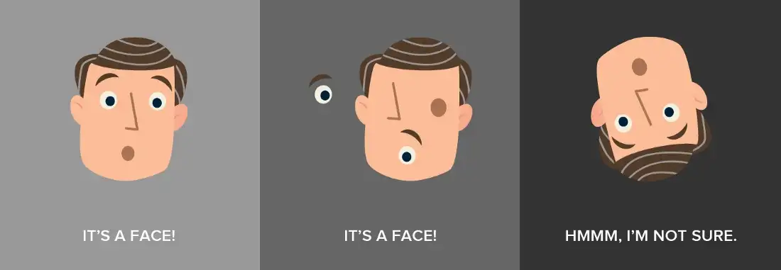
Take the left-most image as the reference image, we have trained our current ConvNet on it. Now, as per the 1st disadvantage, when we rotate the image, the filters extracting the important information such as eyes, nose, and mouth may not be aligned with their position in the right-most image. And as the network has not seen any image like that in its training, it hasn’t generalized well so it makes a wrong prediction.
Now for the 2nd disadvantage, consider the image in the middle. The overall orientation of the face is similar but we’ve swapped the locations of some of the features. Here, the network is able to recognize some of the features, if not all, with the respective filters placed in its space, and thus it classifies it as a face.
Disadvantage #3
The third and final flaw is again due to the design of these ConvNets. The way they route information to the higher layers creates a broader receptive field for these upper layers. Instead of routing all the information through all the layers, networks can be made selective so as to pass the required information to the respective layer.
Our brain functions in a similar manner, we have different lobes that have their own specific function at which they are good. Similarly, routing the feature of an eye only to the part that detects face is much more intuitive rather than sending it to the filter detecting animals, chairs, etc.
CapsuleNets are inspired by this phenomenon, like our brain it works using the concept of ‘inverse graphics’. Let’s understand the working of CapsuleNets using an example. The overall architecture is divided into three sub-parts:
- Primary Capsules
- Higher Layer Capsules
- Loss calculation
We’ll see the usage of each of the sub-part in the example.
Before we begin, we will learn about the basic building block of CapsuleNets, i.e. the Capsule, and how it is different from a neuron. For all other networks, we have a concept of a neuron that resembles the one found in our brain. It takes a set of inputs, weighs them using its learned weights, and then applies an activation function on top of it to build complexity into the model.
Capsule does similar things, but the main difference lies in the output of both the blocks. Capsule outputs a vector instead of a scalar quantity like neurons. This vector carries information about the orientation of the object inside the image. If you rotate the object and/or the image, this vector representation would be simultaneously affected it.
Primary Capsules
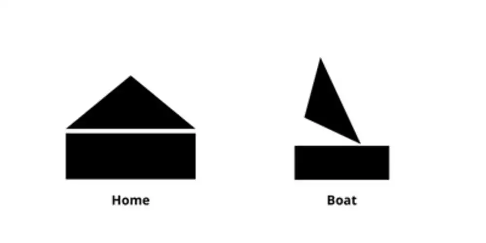
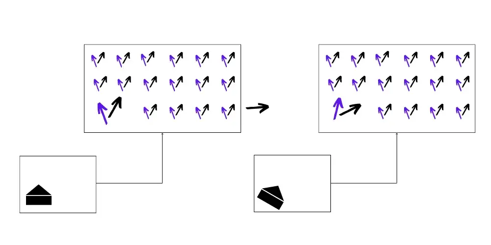
Consider the image above. We can say that the above images are made up of two fundamental parts, a triangle, and a rectangle. Now suppose that we initialize the Primary Capsule layer with 200 capsules, 100 representing the rectangle and the other 100 for the triangle.
They are distributed such that they cover the whole image. The output of each of these capsules is represented using arrows in the below image; black arrows represent the rectangle’s output and the blue ones for a triangle. To decide if a particular object is present or not, we focus on the length of those arrows while their pose gives us information about the orientation of that particular object (position, scale, rotation, and so on).
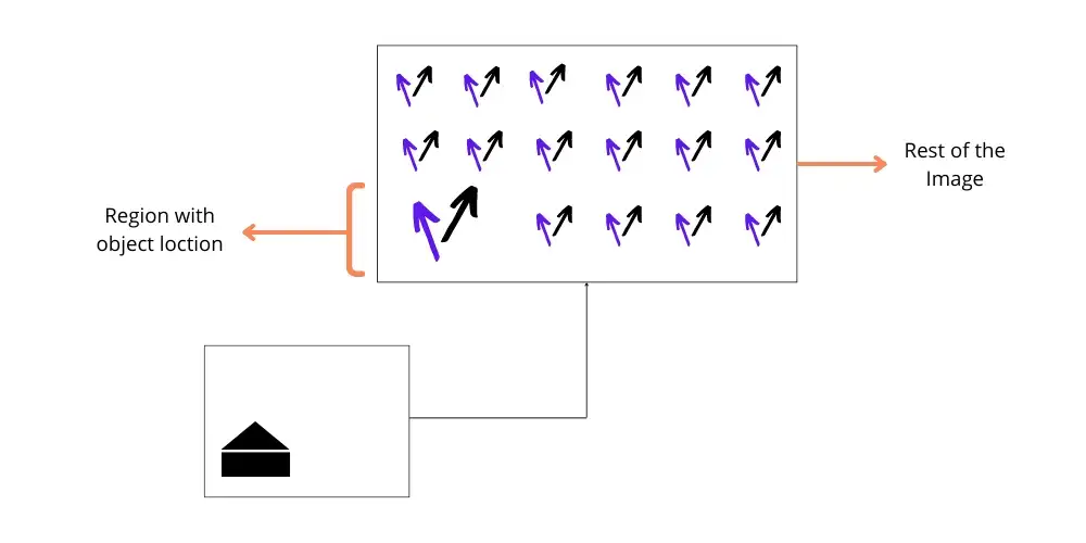
These capsules also follow the property of equivariance, i.e. for a slight change in the position/orientation of the object, we’ll see a corresponding change in the arrows representing these objects. This helps CapsuleNet to locate the object in the image and have precise information regarding the pose parameters.
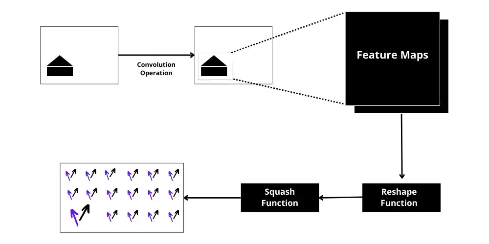
To achieve this, the Primary Capsule layer goes through three different phases:
i) Convolution
ii) Reshape
iii) Squash function
We take the image and process it through Convolution layers to get output feature maps. We then reshape those feature maps.
In our example, let’s consider we got 50 feature maps as output, we reshape them to two vectors of 25 dimensions (50 = 25*2) for every location in the image. Each vector represents one of the two fundamental shapes. These values now can be inferred as the probability of each of the fundamental shapes present or not at a particular location in the image, but to do so they must have their lengths between 0 to 1. To achieve this, we apply the squash function. It basically takes the vector and applies the norm and then a non-linear function to maintain its length between 0 and 1.
So, till now we have the information about the presence of the fundamental shapes in the image. We now need to take this information and infer if it’s a boat or a house. For that, we move to the next layer in CapsuleNet — Higher Layers.
Higher Layers
The next step is the function of Higher layers. But before we jump into them, primary layers have one more function to do. After the squash output, the primary layers also try to predict the output of each of the higher layers. We had 100 capsules for rectangles and 100 for triangles which will give some predictions, supposing that the higher layer has two capsules, one for house and one for boat, these predictions are made w.r.t and the orientation of the shapes found.
Due to the extra information on the pose, the capsules will be able to get to a consensus that the object present can be a boat. This is called routing by agreement. Due to this, the signals are now only sent to the higher level capsule representing the boat and not the other one.
Now, the work of the higher layer begins, even though the primary layers predicted some output for the higher layer, it still needs to predict its own output and validate the same. Initially, the higher layers set the routing weights which are used by the lower layers to route the image signal. It does so by calculating its own output and then validates the output by the lower layers. Based on the similarity of both the predictions, the weights are updated.
Also, after we get the output from the higher layers, we can add a third layer on top of the higher layer which will be a layer of neurons to classify the image based on the vector output it’ll receive.
Wrap Up!
In the article, we saw the working of a CapsuleNet and the intuition that gave birth to this concept. Starting from the drawbacks of CNNs, we built towards their solutions and how CapsuleNets can be a viable alternative for them.
Although intuition and algorithms seem to do well it had their own cons when it comes to reality.
- Due to the dynamic routing and a large number of capsules, the computation becomes heavy and demands a higher computational resource.
- It also suffers from the problem of crowding when two objects of the same type are placed close to one another.
Despite these, CapsuleNets serve as a promising approach for the community and thus can be further improved upon.
Hope the article was able to clearly shed some light on the overall concept and helped you gain a deeper understanding of CapsuleNets. Stay tuned for more such pieces in the future. Au Revoir!
