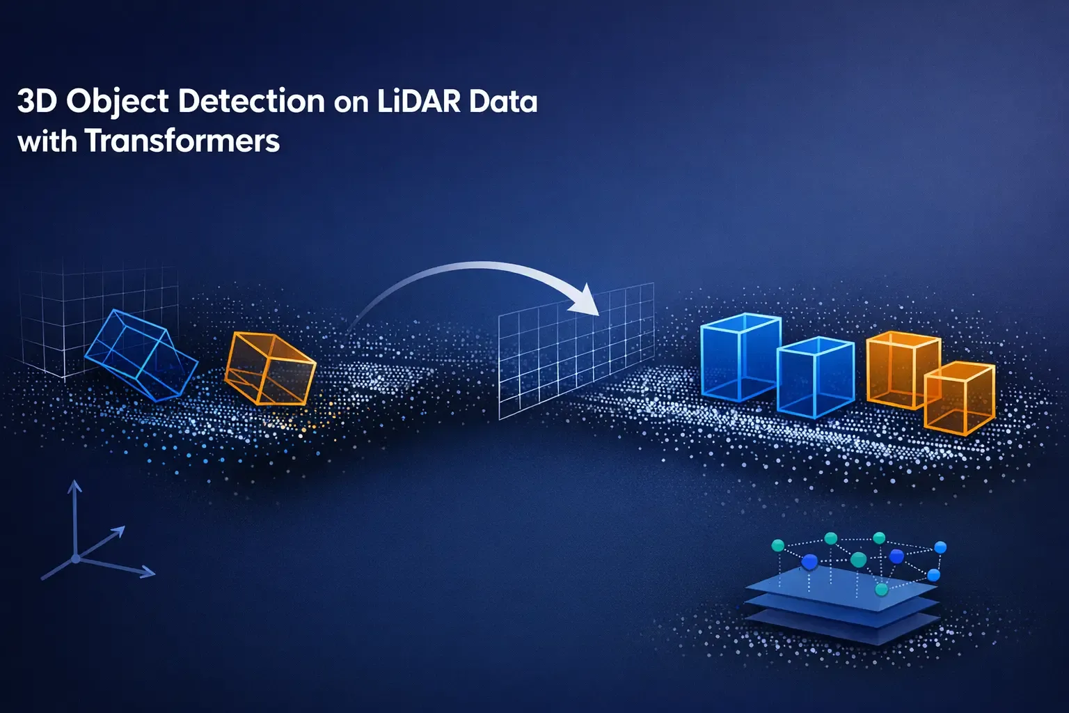
3D Object Detection on LiDAR Data with Transformers
Contributors: Ashwini Rao
In our previous blog, we explored the basics of 3D point cloud data — what it is, how it’s collected using LiDAR and depth sensors, and how different coordinate systems represent it. It gave us an understanding of the raw data representation, how to load & visualize them, the next step is to use these point clouds in the tasks like 3D object detection.
Applications of 3d object detection are spreaded across multiple domains like AR/VR, robotics & autonomous driving.. Traditional approaches use convolutional neural networks (CNNs) or voxel-based architectures. However, with the success of Transformers in vision tasks, researchers have extended these ideas to the 3D domain.
One such model is 3DETR. In this blog, we’ll see how 3DETR can be adapted for outdoor LiDAR dataset — specifically the KITTI dataset — and the various challenges involved in preprocessing, coordinate transformations, and augmentations.
3DETR
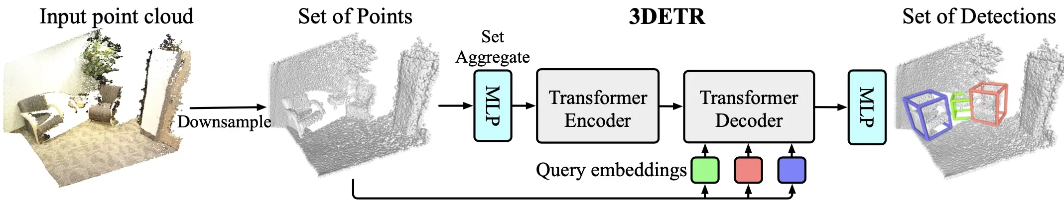
It is also know as “3D Detection Transformer”, used for 3D object detection tasks. It is an end-to-end transformer based model. In contrast to DETR, 3DETR only uses Transformers that have been trained from scratch and does not use a ConvNet backbone. Since 3D point clouds work well with set-based structures like the transformer, it makes use of them directly. There could be millions of input cloud points, to reduce them a single downsampling (Farthest Point Sampling) procedure is used. It uses Fourier positional embeddings in the decoder and non-parametric searches. They demonstrate that by masking the self-attention, 3DETR can readily absorb 3D specific inductive biases (local aggregation matters more than global aggregation) to further enhance its performance.
Datasets
3DETR was originally trained on two indoor datasets:
References
Why Coordinate Systems Matter
When moving from indoor datasets (like SUN RGB-D and ScanNet) to outdoor datasets (like KITTI), one of the biggest challenges is the difference in coordinate systems used by sensors. RGB-D cameras, LiDAR scanners, and depth sensors all define object positions in their own reference frames. To train a unified 3D object detection model, we need a clear understanding of these coordinate systems and how to transform data between them. This leads us to the next section.
Different coordinate systems
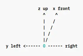
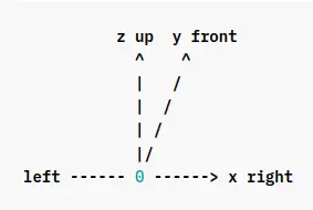
There are tons of different datasets & sensors but for 3D Object detection task, there are three coordinate systems:
Yaw Angle
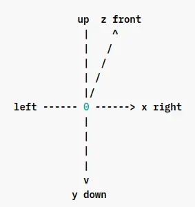
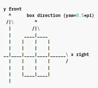
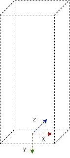
Another important property of 3D objects is Yaw angle. It’s rotation of an object around it’s vertical axis. There is an axis called the gravity axis in object detection, and a reference direction which is on the plane perpendicular to the gravity axis.
Yaw angles:
- Reference Direction: 0
- Other Directions: Angle with the reference direction
Below example shows:
- y-axis as the gravity axis
- x-axis as the reference direction
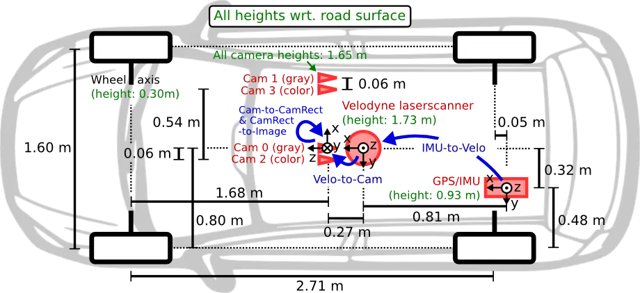
KITTI Dataset
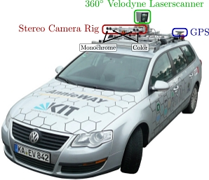
One of the most widely used benchmarks for research in autonomous driving. It was released by the Karlsruhe Institute of Technology and Toyota Technological Institute & that is where the name KITTI comes from.
As shown below different sensors (GPS/IMU, RGB/Grayscale Cameras, Rotating LiDAR) were mounted on a car to collect the data.
It can be used for multiple tasks like:
- Object Tracking
- 3D object detection
- 2D object detection
- Visual odometry
- Optical flow
- Stereo vision.
For 3D object detection, KITTI includes synchronized RGB images, LiDAR point clouds, and ground-truth bounding boxes for objects such as cars, pedestrians, and cyclists.
Now, we’ll study the dataset in the setting of 3D object detection.
3D object detection benchmark:
- Number of training data: 7481
- Number of testing data: 7518
- Total annotated objects: 80256
Structure:
- Calibration Files (.txt)
- Images (RGB + Gray) (.webp)
- Point Cloud Data (.bin)
- Labels (.txt)
Coordinate System:
There are three different sensors & hence three different coordinate systems:
| Sensor | x-axis direction | y-axis direction | z-axis direction |
|---|---|---|---|
| Camera | Right | Down | Forward |
| LiDAR | Forward | Left | Up |
| GPS / IMU | Forward | Left | Up |
Ground Truth Annotations:
The ground truth annotations are given for frames captured from left RGB camera (id-2) & are in the camera coordinate system. To train a model in LiDAR coordinate space, these annotations need to be transformed to LiDAR space. These conversion matrices are given in calibration file for each frame.
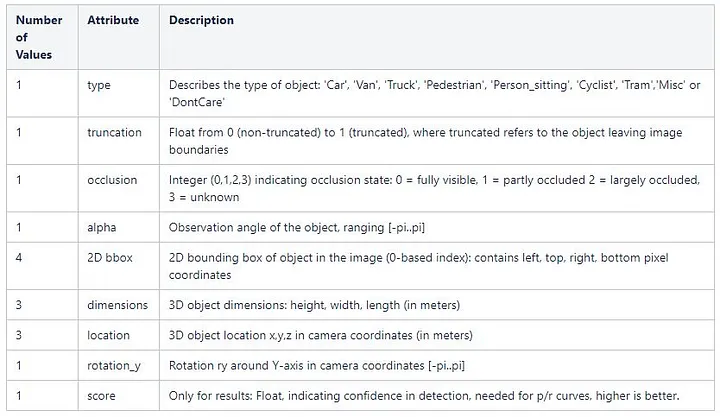
Source: KITTI GT Details
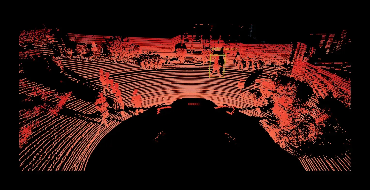
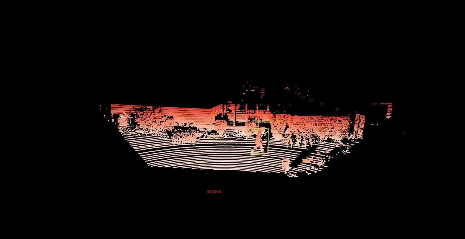
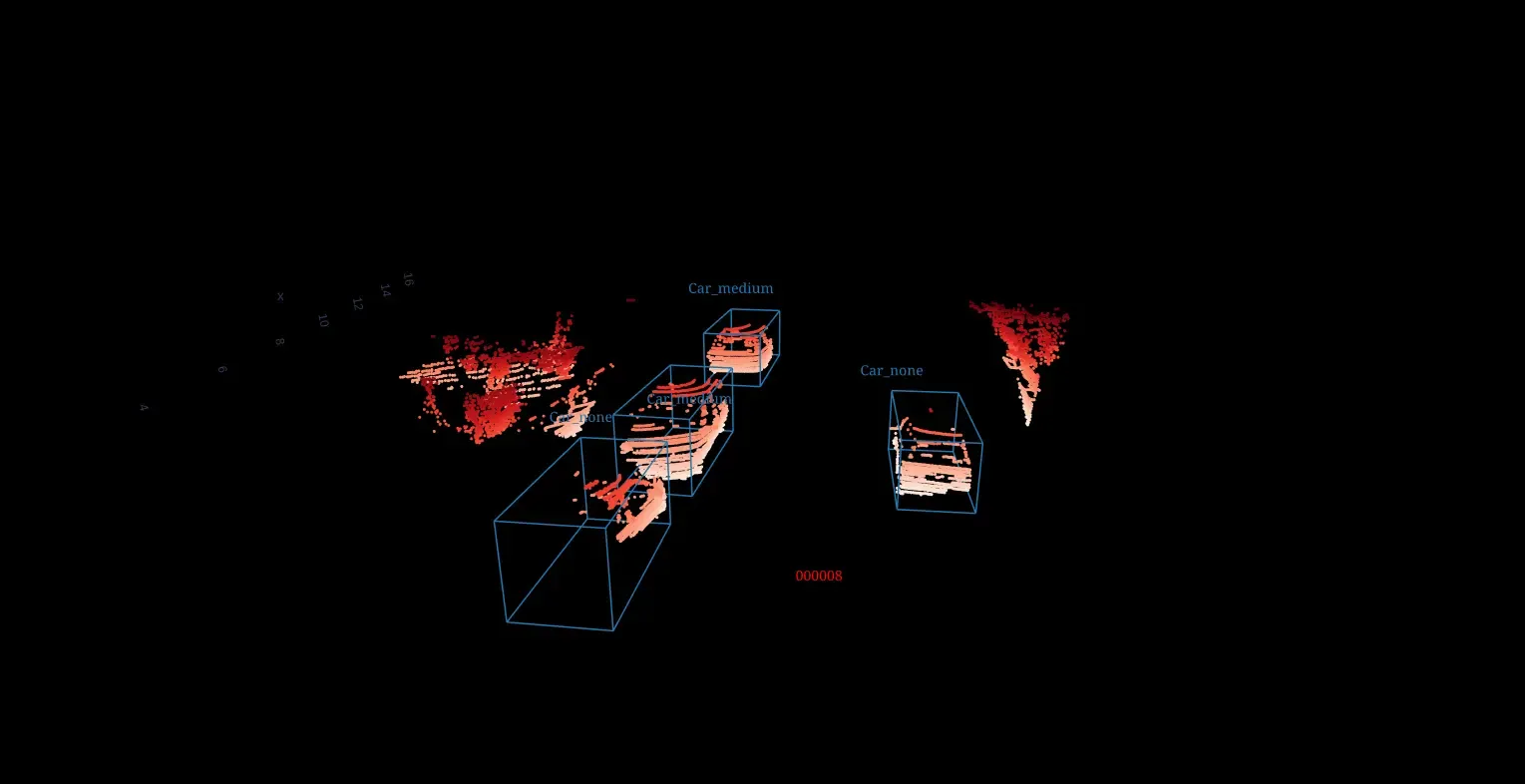
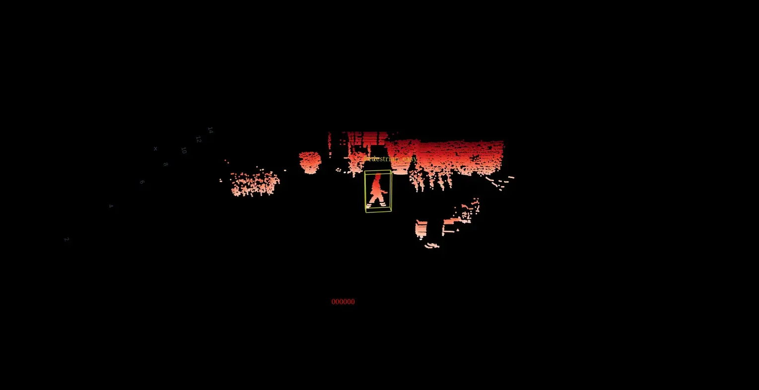
Dataset Visualization
Here we will visualize a couple of point clouds with annotations.
# Load Dataset

print(f"Total Samples: {len(dataset)}")
Total Samples: 21
3DETR Changes for KITTI
We wanted to experiment on 3DETR with KITTI dataset. 3DETR was trained on indoor datasets but KITTI is an outdoor dataset. There are major differences between these datasets in terms of object types, sizes, point cloud density & specifically the coordinate system. Coordinate system differs because of the use of different depth cameras & LiDAR sensors to collect this data.
We have only used LiDAR data and not the images from the KITTI dataset for this experiment.
KITTI Point cloud data is in the above LiDAR coordinate system. Wherein the SUN RGB-D point cloud data is in camera coordinate system. As 3DETR codebase was developed for camera coordinate system, there were some changes needed to be made to make it work for KITTI. Along with this, will also go through the data processing steps for KITTI dataset.
Changes made to original 3DETR:
- Dataset file to pre-process & load data
- As 3DETR was trained on indoor datasets having different coordinate system than KITTI dataset
- BBox pre-processing
- IOU / GIOU calculation
- Heavy Augmentations:
- Random Flipping - X
- Random Flipping - Y
- Random Rotation along Z-axis
- Random Scaling
- Random Translation
- Random Jitter
- Random Dropout
- Random Cuboid Cropping
- Random Ground Truth Pasting
- Gradient Accumulation
- ML Flow tracking
Data Preprocessing for 3DETR
3DETR Input:
- Point Cloud
- Min-Max Range of this point cloud
3DETR Output:
- Classification Logits (Including No-Object)
- Box Center Offsets
- Normalized Box Size
- Angle Logits
- Normalized Angle Residual
Let’s see how to prepare this.
Dataset Loading
from lexper.datasets import KITTIDatasetConfig, KITTIDetectionDataset

dataset_config = KITTIDatasetConfig()
dataset = KITTIDetectionDataset(
    dataset_config=dataset_config,
    split_set="trainval",
    root_dir="lexper/data/kitti",
    augment=False,
)
Point Cloud Visualization Function
def display_raw_point_cloud(
    dataset_config: KITTIDatasetConfig,
    dataset: KITTIDetectionDataset,
    index: int,
    fov: bool = False,
    ground_points_remover: GroundRemover = None,
    remove_ground_points: bool = False,
    radius_filtering: bool = False,
) -> None:

    # Because there is internal radius based filtering in ground point removal
    if remove_ground_points and not radius_filtering:
        radius_filtering = True

    # get filename
    filename = dataset.filenames[index]

    # read point cloud
    point_cloud = np.fromfile(str(dataset.raw_velodyne_dir / f"{filename}.bin"), dtype=np.float32).reshape(-1, 4)[:, :3]

    # read bboxes
    bboxes = dataset._read_bboxes(name=filename)
    corners = dataset_config.box_parametrization_to_corners_np(centers=bboxes[:, :3], sizes=bboxes[:, 3:6], angles=bboxes[:, 6])

    # read calibration file
    calibration = dataset._read_calibration(name=filename)

    # FOV filtering
    if fov:
        point_cloud = dataset._filter_fov_points(points_3d=point_cloud, calibration=calibration)

    # Ground Points removal
    if remove_ground_points:
        point_cloud = ground_points_remover(point_cloud)

    # Radius Filtering
    if radius_filtering:
        distances = np.linalg.norm(point_cloud[:, :2], ord=2, axis=1)
        point_cloud = point_cloud[distances <= dataset.radius]

    # plot data
    fig = get_figure(rows=1, cols=1)
    plot_point_cloud(data=point_cloud, name=dataset.filenames[index], fig=fig)

    # plot bboxes
    for idx in range(corners.shape[0]):
        if radius_filtering:
            distance = np.linalg.norm(bboxes[idx, :2], ord=2, axis=1)
            if distance > dataset.radius:
                continue
        name = dataset_config.class2type[bboxes[idx, 7]]
        difficulty = dataset_config.difficulty_map[bboxes[idx, 8]]
        plot_3d_bbox(points_3d=corners[idx], name=name, fig=fig, extra_text=difficulty, row=1, col=1)

    fig.show()
Preprocessing Steps
Coordinate Transformation for 3D Boxes
KITTI Annotations for 3D Objects are in rectified camera coordinate system. As we are training 3DETR in LiDAR Coordinate system we need these annotations to be converted to LiDAR coordinate system. Here are the steps to achieve this:
Source: 3D Box
- Get axis aligned corners of the bounding box in rectified camera space using
dimensionsof the boxe. - Shift & Rotate (clockwise on y-axis) this box in rectified camera space using
location&rotation_y. - Project these corners from rectified camera space to reference camera space using inverse of
R0_rectmatrix. - Project these corners from reference camera space to LiDAR space using inverse of
Tr_velo_to_camrigid transformation matrix. - Convert the
rotation_yvalue to LiDAR space by negating it. - Map the object
typeto integer value. - Calculate the
difficultyof the object based on the below mentioned parameters:- Easy: Min. bounding box height: 40 Px, Max. occlusion level: Fully visible, Max. truncation: 15 %
- Moderate: Min. bounding box height: 25 Px, Max. occlusion level: Partly occluded, Max. truncation: 30 %
- Hard: Min. bounding box height: 25 Px, Max. occlusion level: Difficult to see, Max. truncation: 50 %
This way will get all the 3D annotations in LiDAR space. We will save these converted bboxes in cx, cy, cz, w, l, h, rot_z, cls, difficulty format as a .npy file. This will reduce the pre-processing time at the time of training.
Point Cloud Pre-processing
We have full 360 view of the point cloud but the annotations are only for the objects apprearing in camera field-of-view. As our goal is to only use the lidar data for object detecion, the far objects having only a few points would be confusing for the model. Also as visualized above we have a lot of points for ground appearing in the point cloud. Taking these things into consideration, here are the preprocessing steps employed for point cloud:
FOV Filtering
- Using
Tr_velo_to_cammatrix, project the point cloud to reference camera space. - Using
R0_rectmatrix, project the point cloud to rectified camera space. - Using
P0matrix, project the point cloud to camera space. - Filter out the points falling outside of the image dimensions. Now this will also have the points at the backside of the mounted sensor too.
- Filter out the points having
x < 0(in lidar space).
Radius Filtering
- Filter out the points falling outside of the pre-configured radius (ex: 15 meters):
- Lidar mount location is the origin. Calculate the distances of the points in 2D space (XY Plane) from the origin.
- Filter out the points having distance more than the
radius.
Ground Points Removal
- Divide the XY plane in n_segments. Segment size: 2pi / n_segments
- Divide each segment in n_bins using r_min and r_max. Bin size: (r_max-r_min) / n_bins
- Add the above data to the points to make them 5D points.
- For each segment:
- Find the point having minimum height for each bin.
- Iterate over these points and fit lines meeting pre-configured conditions.
- For each segment:
- Determine the points’ distances from the lines fitted to this segment and adjacent segments.
- Mark a point as the ground point if the distance between it and any line falls within the threshold.
- Return the non-ground points.
- We used this repository for this but with these fixes:
- Radius based filtering was wrong (function:
filter_out_range). Instead of using bin numbers, use the euclidean distance of the point for filtering. - Don’t flip the z-axis as mentioned in the repo’s README. Provide lidar height as -ev value for it to work.
- Radius based filtering was wrong (function:
We observed that the above filtering can result into having 0 points in the point cloud. We can’t pass an empty point cloud to the model. For these cases we will add two points (0, 0, 0) and (1, 1, 1).
As these are some heavy computations, we can do these prior to the training & save the processed point clouds which can save us some time.
Box Filtering
- Use the
ignored_classesfilter to remove the boxes. For instance, if we wish to train exclusively on a few classes. - Filter out the boxes using
difficulty. For example. if we want to train only on some specific difficulty levels. - Filter out the boxes with center falling outside of the
radius.
Augmentations
Here are the augmentations added for training:
- Random Flipping - X
- Random Flipping - Y
- Random Rotation along Z-axis
- Random Scaling
- Random Translation
- Random Jitter
- Random Dropout
- Random Cuboid Cropping
- Random Ground Truth Pasting
Will see the visualizations for these augmentations & how they look in a 3D Space!!
Low points Box Filtering
Now, there will be cases when the objects are highly occluded or are partially outside the FOV. Which could result into having a very few points in the box. We will filter out these boxes based on the threshold value.
Ground Truth Preparation
After the above steps we will have the final bounding boxes and the point cloud. We need to convert these to required format for batching & training. Batching requires same input dimensions for the data points. We will pre-configure the number of point cloud points & max-objects for this. We can find these values based on the data-analysis.
- Bin the rotation angle and find it’s residual. Number of bin are pre-configured.
- Sample the configured number of points from the point-cloud.
- Find the min-max range of the point cloud and use it to normalize the box center and dimesions.
- Update the raw angle using the binned and residual value. So that both aligns properly.
- Calculate the box corners using this value of rotation.
- Using the box dimensions calculate the corners with the origin as the center. (Length on the y-axis, height on the z-axis, and width on the x-axis)
- Get the anti-clockwise rotation matrix about the z-axis.
- Rotate the box.
- Transalte it using the original box center.
After these changes, use this dataset to plot and visualize the point cloud and bounding boxes to verify the transformations.
Augmentations Visualizations
Random Cuboid Crop
It involves randomly selecting a cuboid-shaped region within the scene and cropping the point cloud to only retain points within that cuboid. It’s similar to random cropping in 2D Images. It simulates truncation of the scene & helps model generalize.
Also, as it is applied before the point sampling, we get more dense representation of the points in the cropped cube.
How it works ??
- First the dimesions of the cuboid are calculated based on the pre-configured values
- A point is randomly selected from the point cloud as the center
- A cube is created around this
- Number of points falling inside this is calculated
- If it is meeting the minimum points requirement:
- Check if there is atleast one object center falling inside this
- If there is one object then this crop is returned
- If not then will iter this process again
- If it is not meeting the minimum points requirement then this process is repeated again
Currently max retries is set to 100
Example
Original Point Cloud:
Cropped Cuboid:
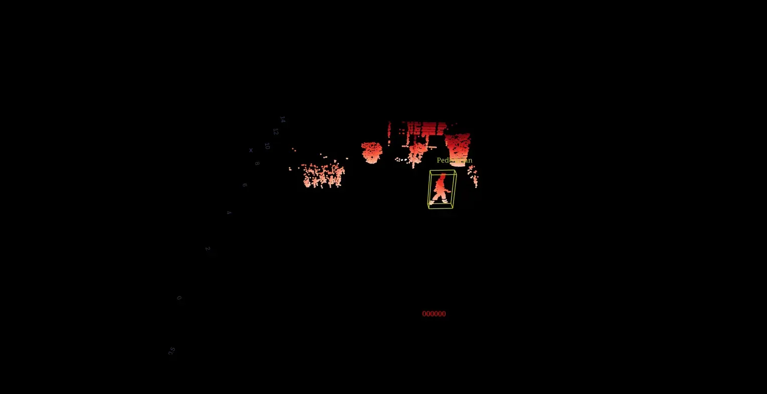
Ground Truth Pasting
Ground Truth Pasting is a data augmentation technique used in 3D object detection where labeled object instances (ground truth boxes and their associated points) are copied from one scene and pasted into another. This method artificially increases object diversity, density in training samples & new object interactions without needing new annotations.
How it works ??
- While preparing the current point cloud another point cloud is randomly selected
- Iterate over the objects in this point cloud
- Select the object based on the set probability
- Extract points inside this box
- Normalize the points
- Randomly rotate these points
- Iterate till max retries
- Randomly select a center between the point cloud range (not from the cloud points)
- Create a box around this center using the slected box dimensions & new rotation angle
- Get the number of points falling inside this box
- If number of points is exceeding the threshold value
- Iterate again
- If not then check if it is not overlapping too much with existing objects
- If not then paste the points of this box in the point cloud
- If it is overlapping too much then re-iterate
Max retries is set to 5
Example
Original Point Cloud:
Ground Truth Pasting - 1
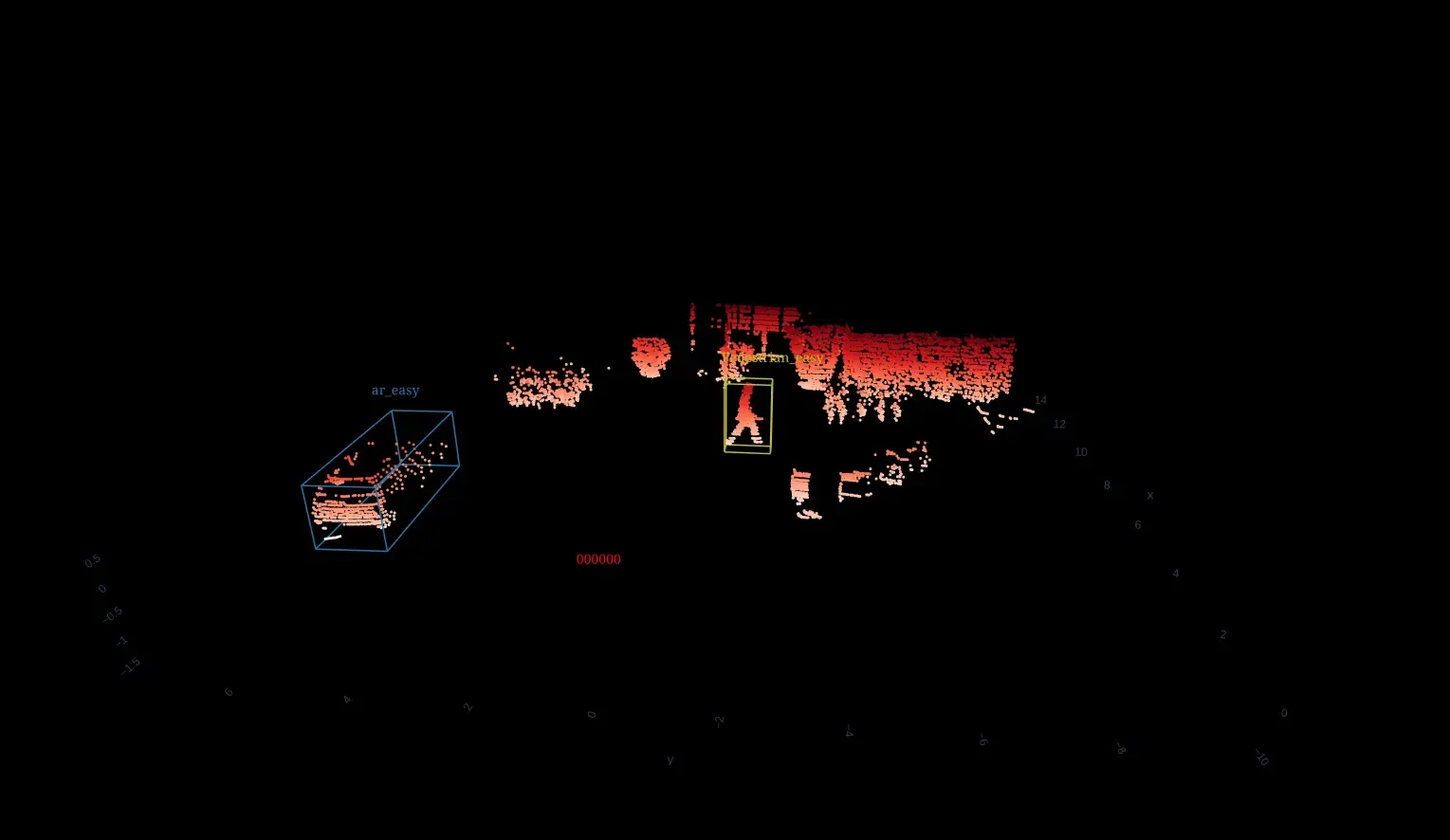
In the below example a car got pasted on the left side of the scene:
Ground Truth Pasting - 2
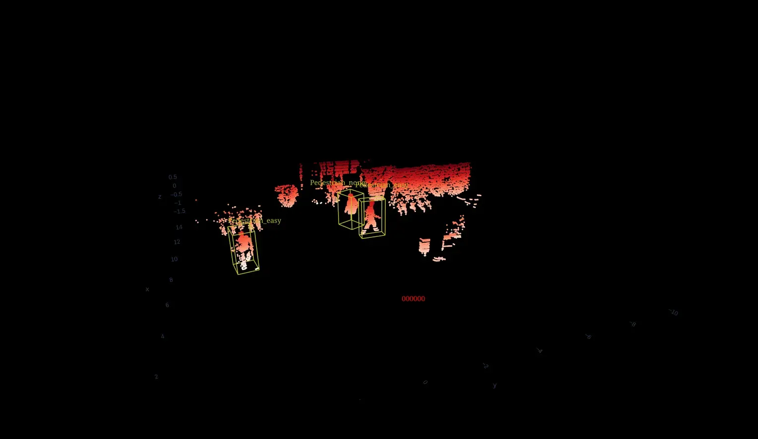
Two pedestrians got pasted in the scene:
Training Setup
- GPU: Nvidia Titan XP
- Classes: Car, Pedestrian, Cyclist
- Per Iteration time: 0.22s
- Memory Occupancy: ~6 GB
Training arguments for 3DETR on KITTI Dataset:
Script to run main.py with the below arguments:
python3 main.py \
    --dataset_name kitti \
    --dataset_root_dir </path/to/kitti_dataset/> \
    --max_epoch 1200 \
    --checkpoint_dir </path/to/store/output/> \
    --batchsize_per_gpu 2 \
    --accumulation_steps 4 \
    --preenc_npoints 3072 \
    --nqueries 128 \
    --base_lr 7e-4 \
    --final_lr 1e-6 \
    --matcher_giou_cost 3 \
    --matcher_cls_cost 1 \
    --matcher_center_cost 5 \run
    --matcher_objectness_cost 5 \
    --loss_giou_weight 0 \
    --loss_no_object_weight 0.1 \
    --warm_lr_epochs 9 \
Training files for 3DETR has been modified and we have added the below things:
- MLFlow Tracking
- Gradient Accumulation
Training Results
Will compare two results, one with no preprocessing and custom changes done on 3detr & other with all the custom changes done which we saw above.
Results without custom changes
| IOU Threshold | Car AP | Pedestrian AP | Cyclist AP | mAP |
|---|---|---|---|---|
| 0.25 | 1.81 | 0.11 | 0.0 | 0.64 |
| 0.5 | 0.1 | 0.0 | 0.0 | 0.03 |
Our Best Run
We used all the augmentations mentioned above along with the gradient accumulation and got the below results:
| IOU Threshold | Car AP | Pedestrian AP | Cyclist AP | mAP |
|---|---|---|---|---|
| 0.25 | 89.5 | 70.56 | 69.44 | 76.5 |
| 0.5 | 66.18 | 15.65 | 22.03 | 34.62 |
Conclusion
With some modifications in the 3DETR which was trained on indoor datasets, we were able to train it for outdoor KITTI dataset.